


Home ||| Art ||| Programming
Modding
This downloadable content was created as a means to showcase multiple disciplines: Programming, Art, Animation and Game Design.


Home ||| Art ||| Programming
Raster to Vector
Introduction
I created this project while working at a data company. While I was there, it became necessary to come up with a way to convert the raster files we were downloading into vector files for use in QGIS, which is a program for displaying geographical data.
The Problem
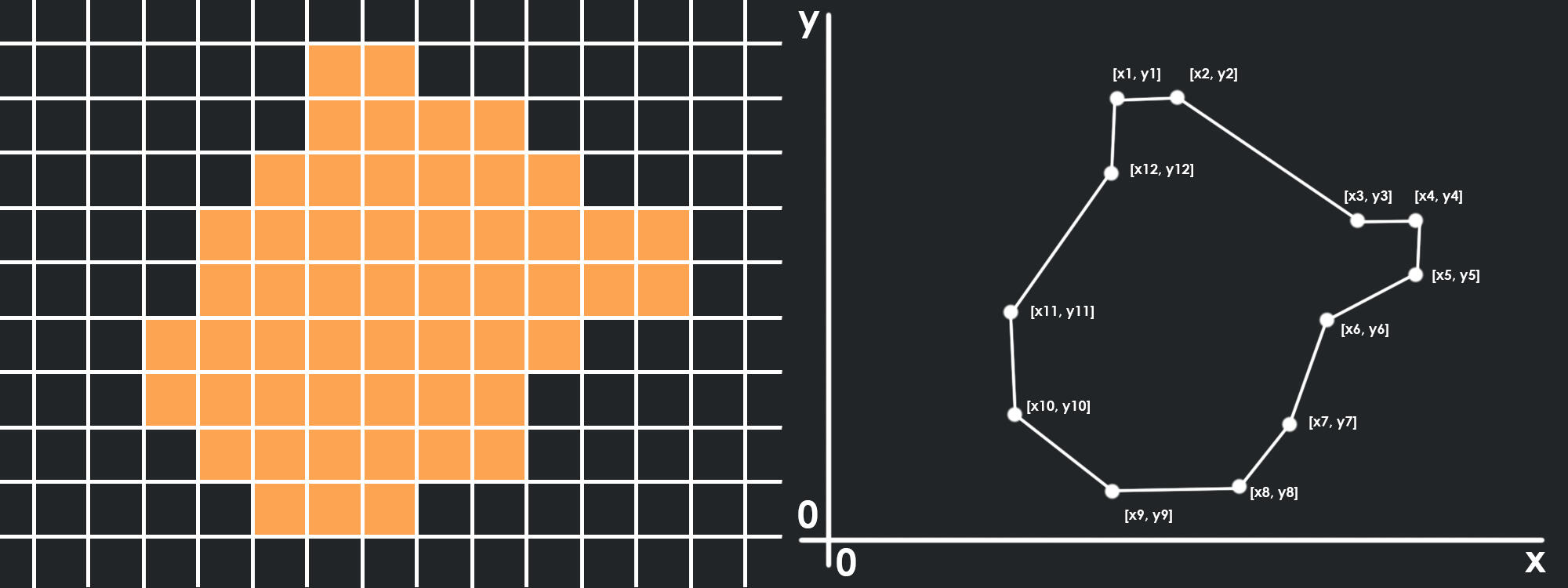
Raster data takes the form of a grid, with each cell containing a value. Vector data is usually much smaller, in this case it is just a list of X,Y coordinates that can be connected by a line to form a shape. The hardest part of the conversion from raster to vector is determining the order of the coordinates, as they must be ordered from start to finish in order to connect them correctly.
The Solution
At the time, I didn't know much about graphics programming and I came up with a CPU bound solution. First, the image is scanned line by line, and each line is divided into segments depending on the colour of each pixel, like so:

Then, for each colour, we create an index for a list of shape objects. Starting with the first line from our raster image, create shapes for each segment found and put those shapes in their corresponding index.For each subsequent line, we compare the segments in the line to the shapes we are building. Each shape keeps track of the last segment added. If the segment we are comparing connects to the last segment added in any of the shapes, we add that segment to the shape. In this way, we build each shape line by line.

As we build each shape, we keep track of the coordinates of each segment. Each segment consists of a pair of X, Y coordinates (x1, y1, x2, y1. y is always the same since it is on the same line).A shape can be described as an equal number of coordinate lists. This means that we can trace a line up and down a shape, keeping track of the coordinates along the way:

This means for every “down” list, there is an “up” list as well. Each shape in our collection has a list of these down and up lists. When we add a segment to a shape, we add the left coordinate of the segment to the down list, and the right coordinate to the up list. In doing so, we keep track of the order of coordinates to pass to the function to make our vector shape.Once every line has been read, parsed and sorted into shapes, we simply build a string of coordinates for each shape, starting at the top of its first down list and ending at the top of its last up list.
Edge Cases
As we add segments, we need to deal with certain cases that happen when a segment does not connect to just one segment above it. If a segment does not connect to anything, we start a new shape.If a segment connects to two other segments, it is either a merge or a loop. In the case of a merge, the segment has connected to two or more shapes. These shapes need to be merged together and their lists combined.

In the case of a segment connecting to two or more segments that belong to the same shape, a loop is created. The shape has a shape within it or a hole, and the inner edges of the loop become disconnected and form their own shape.

Home ||| Pixel Art ||| Programming
Octree Boids

Introduction
This project was done in my final year of university as a joint project between myself and Sam Costigan. The forest geometry was made by Sam, while I combined a flocking algorithm with an octree collision algorithm to optimize the calculation between the boids. The project is written in C++ and the graphics are made with the OpenGL library.
Flocking
This is a common algorithm that mimics the behviour of birds. The basic premise is to give boids (which are represented by the triangles) the ability to detect other boids in the area, and then have them maintain cohesion, alignment and separation.

When doing so, the initial implementation looks like this:

I modified the algorithm to have a tree like structure. The boids now only try to maintain cohesion and alignment with the boids that are above them in the tree, with a single boid as the leader.

The boids still all reference each other when checking for separation, creating an (On2) algorithm. For each boid that is added, the total number of boids must be looped over again to check for distance.
Oct-tree
This is where I combine this algorithm with another algorithm that is often used in collision checking. The simulation area is divided into 8 cubes. Each cube tracks how many boids are in it. If the cube contains above a predetermined number of boids (4 in this case), the cube is subdivided into 8 more cubes. These cubes become the child nodes of the cube surrounding it.

Once all the boids have been sorted into their respective nodes, or the node size has reached its limit, the boids only have to check the distance to the sides of the cube they are in, or the other boids in the cube. If it is closer to the side, it has to check the boids in the neighboring nodes, but otherwise it just has to check the boids in its own node.

Home ||| Pixel Art ||| Programming
Solvix
Introduction
Solvix is a tool for simulating 2d fluid dynamics. This tool is a personal project I created to help with improving my knowledge in C++ and graphics programming, as well as provide a convenient way of simulating certain types of animation that are otherwise tedious to do.
Fluid Dynamics
Most GPU fluid simulations like dye, smoke, gas, etc. are driven on implementations of the Navier-Stokes fluid equation. This equation dictates that the fluid field must go through several steps to simulate fluids:
1. Pressure: As forces propagate, they create acceleration in areas of the field they push on
2. Advection: The values in the field must be carried along the force vectors present at their point in the field.
3. Diffusion: Values in the field will bleed into their surroundings, according to the viscosity of the field.
4. External Forces: We must add an injection of values into the field to stimulate it and watch it evolve over time.
Implementation
We do this incrementally to see the fluid move over time. We use a 2D array to hold our values and represent the fluid field. The row and column index of each cell is the X, Y value of the cell. This array is used as a texture (a texture is an array of N dimensions, 2 in this case) for the GPU to work with. In my solution, we have a separate texture to hold the velocity of each cell and the amount of dye in each cell.We do each step in reverse order due to matrix mathematics, with the pressure (step1) after both advection and diffusion in order to clear divergence problems within the field. We start by adding forces that we want to inject into the field

Next we move onto diffusion. Each cell receives value from the surrounding cells, including negative values from surrounding cells that have less value. The amount of value received depends on the rate of diffusion/the viscosity of the field.

For advection, we need to take the velocity of the same cell in the previous increment and trace it backwards. From this position, we need to get the value of the cells surrounding this point and interpolate the average, then write that value to our current cell.

When we make changes to the field with diffusion and advection, we need to make sure that the incompressibility of the fluid is maintained. For instance, if a cell is surrounded by inward forces, those forces cannot have their values consumed by the cell and their components must be evenly distributed. Similarly a cell surrounded by outward forces cannot distribute more than the sum of its value.

In order to remove this imbalance, we need to subtract the divergence from our velocity field to arrive at a divergence – free velocity field. The divergence of a cell is the amount by which it is out of balance. It can be calculated using this method:

The field of divergence is equal to the field of the pressure across the current velocity field. For each cell this equation can be written as:
(p[Left] + p[Right] + p[Up] + p[Down])- 4 * p[Center] = divergence(velocity)
Since P is unknown, we have to solve for every cell in the field at once as a system of simultaneous equations. For efficiency, we use a Jacobi method to solve this. First we rearrange the equation to have P(center) on one side:
p[Center] = (p[Left] + p[Right] + p[Up] + p[Down] – divergence(velocity))/4
Then we find our divergence(velocity) for the last field using the operation in the last image. Now, starting from 0, we repeat this operation enough times to get an accurate answer, i.e: 20. Each time we replace P(center) with the answer we got from the last iteration. At the beginning of the process, P for the left, right, up and down cells will also be 0, but will change over time according to the cells surrounding them, and so on. Eventually, all cells will converge in on the right answer.Now that P has been found, all we have to do is subtract the divergence of P from the current velocity field:
divergence-free Vx = Vx – (p[right] – p[left])
divergence-free Vy = Vy – (p[up] – p[down])
And we get our final velocity field free of divergence. We should do the projecttion step once after diffusion and once after advection to get the most accurate simulation, although in my solution I only do it once after advection and it seems to work fine. We only need to do this step for the velocity field, as the dye field can just store dye as a number as high as it needs to go, until it is distributed later.
Other Additions:
If we add a simple mono-directional force and some dye on top to our simulation, the result can look quite uniform:

In order to add some aesthetic interest, we can add vorticity:

We do this by taking advantage of the divergence of the field to find local areas of curling, and then boosting those the vectors in those areas to exaggerate the curls. Since we need to use divergence, we do this step after the diffusion step, before we clear the divergence.First we find the divergence of each cell, like before. We then save this value into a texture to create a divergence field. Then in our original velocity field, we can find the divergence numbers arround each cell and use them to modifiy the velocity in the cell, using this method:
dx:=abs(curl(x + 0, y - 1)) - abs(curl(x + 0, y + 1));
 dy:=abs(curl(x + 1, y + 0)) - abs(curl(x - 1, y + 0));
 len:=sqrt(sqr(dx)+sqr(dy))+1e-5;
 dx:=vorticity/len*dx;
 dy:=vorticity/len*dy;
 xvelocity[x,y]:=xvelocity[x,y]+timestep*curl(x,y)*dx);
 yvelocity[x,y]:=yvelocity[x,y]+timestep*curl(x,y)*dy);
Finally, I made this project with usability in mind. The imgui library is a common developer UI and I used it here to add controls to the simulation. I also used a library called gif-h to export simulations as a .gif recording for use in other programs to trace over. You can watch the video at the top of the page for a full explanation of the controls.